Advertisement
Quick Links
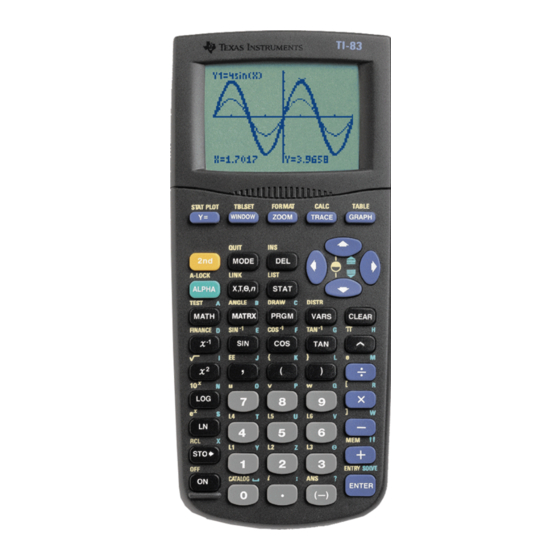
TI-83 Graphing Calculator Manual to Accompany
Precalculus Graphing and Data Analysis
How to Use This Manual
This manual is meant to provide users of the text with the keystrokes necessary to
obtain the output provided by the TI-83 graphing calculator as that obtained in the text.
This manual by no means covers all of the features of this calculator.
In addition, once a particular feature is introduced, it will not be discussed again.
For example, graphing is introduced in Section 1.2, therefore, when graphing is again
required in Section 6.4, the keystrokes required are not reviewed and are assumed to be
known.
Introduction to the TI-83
Before learning how to use the TI83 as a graphing calculator, an introduction to
the TI83 as a scientific calculator may be worthwhile. In this introduction, basic
calculator skills will be discussed.
Turning the Calculator On and Off
The ON button is located in the
lower left hand corner of the keyboard. To
turn the calculator off, press the 2
and then the ON button. Notice that all 2
functions are in yellow on the keyboard.
An Introduction to the TI83 Keyboard
If you look at the bottom portion of the TI83, you should recognize that it looks
similar to a standard scientific calculator. This portion of the calculator is enclosed in the
box shown on the calculator above.
nd
button
nd
ON button
nd
2
Function
Advertisement

Related Manuals for Texas Instruments TI-83


Summary of Contents for Texas Instruments TI-83
- Page 1 This manual is meant to provide users of the text with the keystrokes necessary to obtain the output provided by the TI-83 graphing calculator as that obtained in the text. This manual by no means covers all of the features of this calculator.
- Page 2 ENTER. So, to perform the operation 4 + 5, simply type 4 and hit ENTER. 3 − The TI-83 is aware of the order of operations, so to evaluate: simply type: 3 ( 4 - 5 * 6 ) and hit ENTER.
- Page 3 Alternatively, you could use the caret key with the “negative” button. Notice the TI-83 automatically puts the solution in decimal form. Should you want your answer to be in a fraction, use the FRAC option under the MATH menu. For example, to compute the reciprocal of 5 with the solution in fraction −...
- Page 4 We wish to access option 1:Frac . Since this is the option currently highlighted, we select it by pressing ENTER or pressing the number 1 on the keyboard. You should obtain the following: Press ENTER to see the result: Suppose we computed the reciprocal of 5 without using the FRAC option as follows: We then realize that we wanted our answer as a fraction.
- Page 5 The calculator automatically stores the most recent output in a memory locator call Ans. So, the calculator will take the output in Ans and convert it to a fraction! NOTE: Ans can also be retrieved using 2 and the “negative” button. RADICALS You should see the square root ( ) as a 2...
- Page 6 For example to compute log 3, simply press the LOG button followed by a 3 and a close parenthesis and hit ENTER. To compute e , press 2 LN followed by 4 and hit ENTER. TRIGONOMETRIC FUNCTIONS Notice the SIN, COS, and TAN functions. To use these features, we need to know whether our angle is in Degrees or Radians.
- Page 7 The remainder of the manual discusses features as they arise in the text. 1.2 Graphs of Equations Example 3 Graphing an Equation on a Graphing Utility Graph the equation 6 SOLUTION Step 1: Done on page 15. = − Step 2: To enter the expression y into a TI-83. Press Y =...
- Page 8 You should see the following on your screen: The highlighted Plot1 means StatPlot is on. To turn it off use the up arrow to put the cursor on Plot1 and hit enter. Move the cursor back down to Y = and your screen should look like this: In Y , type in the following order (consult the figure for the location of these buttons)
- Page 9 X,T,θ,n This squares the ( - ) quantity preceding it. NOTE: This is not the subtraction sign. This button represents the negative of a number. Your screen should have the following: STEPS 3 and 4: To obtain a graph with the standard viewing window press ZOOM and then select option 6.
- Page 10 GRAPH. In order for the feature to work, you must have at least one equation entered in the Y = menu. Before proceeding to the table, I first want to introduce the TABLESET feature. This is activated by pressing WINDOW on your TI-83. TABLE TaBLeSET After pressing 2 WINDOW, the following should appear.
- Page 11 Now press 2 GRAPH to obtain the following TABLE: You can use the arrows to scroll around the TABLE. Notice that whatever quantity the cursor lies on is displayed in the bottom row of the TABLE. Let's go back to TableSetUp to see the affect of changing the independent variable to ASK.
- Page 12 - 8 using Xmin = -5, Xmax = 5, Xscl = 1, Ymin = -20, Ymax = 10, Yscl = 5. The VALUE feature on a TI-83 evaluates an equation for any value of x and locates the corresponding ordered pair on the graph of the equation. Letting x = 0 allows us to find the y-intercept of the graph of an equation.
- Page 13 Thus, when x = 0, y = -8. We can use the ZERO feature on a TI-83 to determine the x-intercepts of the graph of the equation. Again, go to the CALC menu, but this time select option 2: ZERO.
-
Page 14: Solving Equations
Notice the arrow. This is telling you the calculator will look for an x-intercept to the right of this value. The calculator now wants a RIGHT BOUND - this is a value of x to the right of the x-intercept. Use the left and right arrows to move the cursor somewhere to the right of the x-intercept you wish to approximate and press ENTER. - Page 15 EXAMPLE 2 Using INTERSECT to Approximate Solutions of an Equation Find the solution(s) to the equation 3(x - 2) = 5(x - 1). Round answers to two decimal places. SOLUTION Graph each side of the equation: Y = 3(x - 2); Y = 5(x - 1) using the viewing window Xmin = -4, Xmax = 4, Xscl = 1, Ymin = -15, Ymax = 5, Yscl = 5.
-
Page 16: Solving Inequalities
Again move the cursor near the point of intersection and press ENTER. The screen now displays the following: Simply press ENTER a third time and the screen displays the coordinates of the point of intersection: The solution to the equation is x = -0.5. 3 3 Check: The calculator now has x = -0.5 automatically stored. - Page 17 SOLUTION Graph Y = -5, Y = 3x - 2, and Y = 1 using the viewing window Xmin = -8, Xmax = 8, Xscl = 1, Ymin = -8, Ymax = 4, Yscl = 1. We wish to find the point of intersection between Y and Y and the point of intersection between Y...
- Page 18 The graph of Y is between the graphs of Y and Y for -1 < x < 1. EXAMPLE 9 Solving an Inequality Involving Absolute Value Solve the inequality | x | < 4 SOLUTION Graph Y = | x | and Y = 4.
- Page 19 -4 < x < 4 since the graph of Y is below the graph of Y in this interval. 1.6 Lines Square Screens To get a square screen on the TI-83 press ZOOM and select option 5: ZSquare. ZOOM...
- Page 20 The calculator will automatically graph any equations entered in the Y = menu. A note about ZSquare - it will square the viewing window that is established. You may need to adjust the initial window setting before using ZSquare. 1.7 Scatter Diagrams; Linear Curve Fitting Example 1 Drawing a Scatter Diagram The data listed in Table 9 (see page77) represent the apparent temperature versus relative humidity in a room whose actual temperature is 72...
- Page 21 In L1 we will enter the value of the x-variable (relative humidity). Enter 0, 10, 20, etc. into L1. Use the arrows to move the cursor to L2 and enter the values of the y-variable, apparent temperature. After the data has been entered, press 2 QUIT.
- Page 22 Move the blinking cursor to On and press ENTER. Leave the Type where it is above (if you have a different type selected, use the arrows to highlight the same icon as above and press ENTER). Your Xlist should be L1 and the Ylist should be L2. (If they are not, use the arrows to move the cursor and change them.
- Page 23 If you are wondering what the viewing window is press WINDOW: GRAPH WINDOW You should see the following on your screen: So Xmin = -2.5, etc. You could change this viewing window by typing in any values you wish. To obtain the window used in Figure 17(b), we would let Xmin = -10, Xmax = 110, Xscl = 10, Ymin = 62, Ymax = 78, Yscl = 2.
- Page 24 With the data in L1 as the independent variable and the data in L2 as the dependent variable, press ENTER to obtain the line of best fit. The TI-83 does not automatically provide the user with the correlation coefficient. If you desire this value, you must perform the following steps.
- Page 25 (ax + b) on your HOME SCREEN, press ENTER to obtain the following: Page 103 - Using a Graphing Calculator to Evaluate any Function ( ) = − Use a TI-83 to evaluate the function G x at x = 3. That is, find G(3).
- Page 26 Solution Enter the function into the Y = menu to obtain: Press 2 Quit to exit the Y = menu. You should now be at the HOME screen. To , press VARS and evaluate the function in Y obtain the following screen: Press the right arrow to highlight Y-VARS and obtain the following screen: Select 1: Function by pressing ENTER or 1 to obtain:...
- Page 27 Now press ( to obtain: Hit ENTER to obtain the solution: 2.2 Characteristics of Functions EXAMPLE 5 Using a Graphing Utility to Locate Local Maxima and Minima and to Determine Where a Function is Increasing and Decreasing ( ) = −...
- Page 28 We can see a local maxima occurs near x = -1. The query Left Bound? from the calculator means the TI-83 wants you to select a point somewhere left of the local maxima. Use the arrows to move the cursor...
- Page 29 Once the cursor is to the left of the local maxima, press ENTER. Your screen displays the following: Left Bound Notice two things (1) The arrow indicates the calculator will look for a maximum value to the right of the left bound. (2) The calculator now wants a right bound.
- Page 30 2.3 Library of Functions; Piecewise-defined Functions EXAMPLE 1 Analyzing a Piecewise-defined Function For the following function f, − − ≤ < > (c) Graph f using a graphing utility. SOLUTION Press Y = . After Type the following: −...
- Page 31 Select item 4 as shown below: Continue typing the function to be graphed so that you have the following in the Y= menu. The calculator must be in DOT MODE. Press the MODE button on the keyboard and use the arrows to put the cursor on DOT and press ENTER: Alternatively, we could change the graphing style from the Y = menu by 3 dots indicate...
- Page 32 EXAMPLE 2 Evaluating a Composite Function − Suppose that f x . Find )( ) − Solution Let Y as shown. )( ) To compute on the TI-83, we first need to insert Y on the home screen. Press the VARS button...
- Page 33 VARS You should see the following: Hit the right arrow to highlight Y-VARS. Select option 1: Function by pressing ENTER.
- Page 34 Select Y by pressing ENTER. Y appears on your HOME screen. Press the open parenthesis located directly above the 8 on the keyboard. Repeat the process described above to obtain Y in order to place Y the HOME screen. Press the open parenthesis key again, the number 1 and two close parenthesis and press ENTER.
- Page 35 Press ENTER to get QuadReg on the HOME SCREEN. In L1 we have the independent variable and in L2, we have the dependent variable. In anticipation of graphing the quadratic function of best fit on our scatter diagram, we can perform the following steps to have the calculator automatically store the quadratic function of best fit into Y With QuadReg on the HOME SCREEN, press VARS, scroll right to highlight Y-VARS, select...
- Page 36 3.2 Power Functions; Curve Fitting EXAMPLE 3 Fitting Data to a Power Function In order to find the power function of best fit repeat the steps given for finding the quadratic function of best fit. However, instead of selecting 5:QuadReg, select A:PwrReg.
- Page 37 Function Decimal Point You should now see the following on your HOME screen: Now press ) + ( - 2 + 3 i) and hit ENTER You should see the following on your HOME screen: EXAMPLE 4 Writing the Reciprocal of a Complex Number in Standard Form Write in standard form a + bi;...
- Page 38 Enter the expression 1 / ( 3 + 4 i ) on the HOME screen: SOLUTION To obtain a fraction, press MATH, then select option 1: uFrac under the MATH menu. MATH Hit ENTER to select 1: uFrac. You should see the following on your HOME screen: Press ENTER to obtain the following result:...
- Page 39 5.2 EXPONENTIAL FUNCTIONS EXAMPLE 1 Using a Calculator to Evaluate Powers of 2 Using a calculator, evaluate: SOLUTION On the HOME screen type 2. Now press the caret (^) key. Caret key Finally, type 1.4 as shown: Press ENTER to obtain the result shown in Figure 12. 5.8 Exponential, Logarithmic, and Logistic Curve Fitting EXAMPLE 1 Fitting a Curve to an Exponential Model (a) Using a graphing utility, draw a scatter diagram...
- Page 40 SOLUTION (a) Enter the independent variable (year) in L1 and the dependent variable (price) in L2. The scatter diagram is shown below. Scatter diagrams are discussed in Section 1.7 if you need a review. (b) Press STAT, scroll right to highlight CALC and select 0;ExpReg as shown below: You should obtain the following on your HOME screen Hit ENTER to obtain the following output:...
- Page 41 EXAMPLE 2 Fitting a Curve to a Logarithmic Model To perform logarithmic curve fitting, repeat the steps described above for Exponential curve fitting, but select 9: LnReg as shown below: EXAMPLE 3 Fitting a Curve to a Logistic Growth Model To perform logistic curve fitting, repeat the steps described above for Exponential curve fitting, but select B: Logistic as shown below: NOTE: In order for the output to include the correlation coefficient, r, you must turn...
- Page 42 SOLUTION (a) On the HOME screen type: 50. You should see the following: Now, access the angle menu. On the TI83 Plus, it is above the APPS button as shown: ANGLE Now select 1: You should have the following on your HOME screen:...
- Page 43 Now type 6 to obtain the following: Go back to the angle menu and select item 2: ′ You now have the following on your HOME screen: Type 21. To obtain the double quotes representing the seconds, press ALPHA then the plus sign as shown. ALPHA The double quotes are...
- Page 44 After pressing ENTER you obtain the following result: (c) Type 21.256 on your HOME screen. Then select the angle menu and choose option 4: u DMS You should now have the following on your HOME screen: Press ENTER to obtain the solution.
- Page 45 6.2 TRIGONOMETRIC FUNCTIONS: UNIT CIRCLE APPROACH EXAMPLE 9 Using a Calculator to Approximate the Value of Trigonometric Functions Use a calculator to find the approximate value of: π SOLUTION (a) Set the MODE to degrees. This is done by pressing the MODE button on the calculator.
- Page 46 Now type / 1 2 ) Hit ENTER to obtain the result shown in Figure 32. 6.6 Sinusoidal Graphs; Sinusoidal Curve Fitting EXAMPLE 10 Finding the Sine Function of Best Fit Use a graphing utility to find the sine function of best fit for the data in Table 11 on page 429.
-
Page 47: Polar Coordinates
Find the rectangular coordinates of the points with the following polar coordinates: , 6 π SOLUTION From the HOME screen, access the ANGLE menu (2 APPS on the TI-83 Plus) and select 7: PuRx(. You should have the following on your HOME screen:... - Page 48 Now type 6 , π / 6 ) and hit ENTER to obtain the following: Repeat the process to obtain the y-coordinate, but select 8:PuRy( instead. EXAMPLE 6 Converting from Rectangular Coordinates to Polar Coordinates Find polar coordinates of a point whose rectangular coordinates are (0, 3).
- Page 49 To obtain the angle, repeat the above procedure, but select 6:RuPθ( . 9.2 Polar Equations and Graphs EXAMPLE 4 Graphing a Polar Equation Using a Graphing Utility θ Use a graphing utility to graph the polar equation SOLUTION We must change the MODE of the calculator to POLAR mode. This is done by pressing MODE and using the arrows to put the cursor on POL and pressing ENTER as shown: Now press the Y = button and enter the expression in...
- Page 50 10.7 Plane Curves and Parametric Equations EXAMPLE 2 Graphing a Curve Defined by Parametric Equations Using a Graphing Utility Graph the curve defined by the parametric equations − ≤ ≤ SOLUTION We must first put the calculator into parametric mode. Press the MODE button and use the arrows to highlight PAR and press ENTER: Now press the Y = button.
- Page 51 EXAMPLE 5 Projectile Motion Suppose that Jim hit a golf ball with an initial velocity of 150 feet per second at an angle of 30 to the horizontal. (d) Using a graphing utility, simulate the motion of the golf ball by simultaneously graphing the equations found in part (a).
- Page 52 The augmented matrix of the system is − − − − − To enter this matrix into the TI-83, press the MATRX button. On the TI83+, the MATRX button is Function.
- Page 53 MATRX on the TI83 You should see the following on the screen: To enter the augmented matrix into the calculator, highlight EDIT: After pressing ENTER you obtain the following:...
- Page 54 We wish to enter a 3 by 4 matrix, so press 3 and hit ENTER, then press 4 and hit ENTER. You should see the following on your screen: Now enter the entries of the augmented matrix. You can use the arrows to move around. Notice the bottom of the screen indicates your location within the matrix.
- Page 55 This is the same as FIGURE 7(a) on page 732. To obtain the ref( command, press MATRX and scroll right to highlight MATH. Scroll down to item A:ref(. Select it by pressing ENTER. You should see the following on your home screen: Now select matrix A by pressing MATRX and highlighting matrix A under the name menu.
- Page 56 Now press the close parenthesis ) - this is a 2 function above the number 9. We want our matrix in fractional form, so press MATH and select 1:äFrac. Now press ENTER to obtain the result shown in Figure 7(b). You can scroll right using the arrow key to see the rest of the matrix.
- Page 57 We enter the matrix A. If you don't remember how to enter a matrix, see Section 11.3 of this TI-83 manual. You should have the following in A: Select MATRX, scroll right to highlight MATH. Now select 1:det(. You should have the following on your home screen: Select matrix A by press MATRX and selecting 1:[A] from the NAMES menu.
- Page 58 − − = = To find the value of x, we evaluate det([B])/det([A]) as shown below: 11.5 Matrix Algebra EXAMPLE 3 Adding and Subtracting Matrices − − ...
- Page 59 3) Press MATRX. Under the NAMES menu, select 2. [B] by pressing 2 or highlighting 2 and hitting ENTER. You should have the following on your home screen: 4) Now press ENTER to obtain the result. To find A - B, repeat the above steps, but select the subtraction sign instead of the addition sign.
- Page 60 Find its inverse. SOLUTION Enter the matrix A into your TI-83 as done in Section 11.3. Press MATRX and select matrix [A] so it appears on the home screen as follows: Press the inverse button on your calculator:...
- Page 61 EXAMPLE 15 Using the Inverse Matrix to Solve a System of Linear Equations − + = − Solve the system of equations: SOLUTION Enter the following matrices into your TI-83: 1 1 0 ...
- Page 62 Section 11.8 Systems of Linear Inequalities; Linear Programming EXAMPLE 2 Graphing a Linear Inequality Using a Graphing Utility + − ≤ . Use a graphing utility to graph 3 SOLUTION = − Graph (this is obtained by solving 3x + y - 6 = 0 for y). Use the same viewing window as that used in the text.
- Page 63 Select 6: < by pressing 6 or scrolling down and highlighting 6 and then pressing ENTER. You should now have the following on your home screen: Finally, press 0 and hit ENTER: The 1 as output means the statement is true so that (-1, 2) is a solution to the inequality. Therefore, we shade the side containing (-1, 2).
- Page 64 calculator to shade above the line. Press ENTER one more time and we see the calculator will now shade below the line: Press GRAPH with the line style as shown above to obtain the following graph: 12.1 Sequences EXAMPLE 2 Using a Graphing Utility to Write the First Several Terms of a Sequence Use a graphing utility to write the first six terms of the following sequence and graph it.
- Page 65 LIST You will see the following on the HOME screen: Scroll right to highlight OPS and select 5: seq( so you see the following on your HOME screen: The sequence command requires the following input: Seq(function,variable,starting point, ending point, step) Enter the following in your calculator:...
- Page 66 After pressing ENTER, we obtain the following: If you want the terms of the sequence as fractions, press MATH and select 1.4Frac to obtain the following: Press ENTER to obtain the following: If you wish to see the remaining terms in the sequence, use the arrow keys to scroll right.
- Page 67 To graph the sequence, first put the TI83 in sequence mode. This is done by pressing the MODE button: MODE Use the arrows to highlight Seq and press ENTER to select sequence mode. Press Y= to obtain the following: Enter the function in u(n)= as follows:...
- Page 68 NOTE: The variable n is obtained by pressing the X,T,θ,n button. For u(nMin), type the value of the function at n = nMin. Typically, the value of n will be 1 since we require the sequence be defined for positive integers (1,2,3,…). Now set the viewing window by pressing WINDOW.
- Page 69 Select 4: !. You now see the following on your HOME screen: To obtain the result press ENTER. EXAMPLE 7 Using a Graphing Utility to Write the Terms of a Recursively Defined Sequence Use a graphing utility to write down the first five terms of the following recursively defined sequence.
- Page 70 Again, the n is obtained by pressing the X,T,θ,n button. Finally, u(nMin) is set equal to Next, set the viewing window. Since we want the first 5 terms, nMin = 1 and nMax = 5. Now press GRAPH to obtain the figure. To obtain a TABLE of values in the sequence, set up the table as shown below (remember, TBLSET is 2 WINDOW).
- Page 71 We start the table at 1 since the recursive sequence begins at n = 1 and ∆Tbl = 1 because the domain of the sequence is the positive integers. Now press TABLE to obtain: EXAMPLE 12 Using a Graphing Utility to Find the Sum of a Sequence Using a graphing utility, find the sum of the sequence ∑...
- Page 72 Now type the rest of the command line as shown below and press ENTER to obtain the result. NOTE: The sequence command has the following syntax: Seq(function, variable, start, end, step) 12.5 The Binomial Theorem EXAMPLE 1 Evaluating ...
-
Page 73: Permutations And Combinations
Press MATH and highlight PRB and select 3: nCr: You should have the following on your HOME screen: Now type 15 and press ENTER to obtain the result. 13.2 Permutations and Combinations EXAMPLE 5 Computing Permutations Evaluate P(52, 5) SOLUTION From the HOME screen, type 5 2 to obtain the following:... - Page 74 Now press the MATH button and scroll right or left highlighting PRB and select 2:nPr: You should have the following on your HOME screen: Now type 5 and press ENTER obtaining: EXAMPLE 8 Using Formula (2) Evaluate C(52, 5) SOLUTION Use the same procedures as were followed to evaluate P(52, 5) except choose 3: nCr under the MATH, PRB menu.
- Page 75 In order to perform a simulation, we must first set the seed. Typically, I suggest that students use the last four digits of their social security number as the seed. From the HOME screen type the last four digits of your social security number (or any number you wish).
- Page 76 We now want to draw a histogram of the data in L1 so we can determine the number of “1s” and “2s”. Press 2 Y = to access the STAT PLOT menu. Select 1:Plot1. After selecting Plot1 you obtain the following: Histogram Highlight Icon...
- Page 77 Press TRACE and use the right arrow to move the cursor to the first “box”. Hit the right arrow again and you’ll be on the second “box”. You should obtain a result similar (although not the same unless you used the same seed) as shown below: We had 52 “1s”...
- Page 78 The syntax for the numerical derivative of f at x = c is : NDeriv(function, variable, c) 14.5 The Area Problem; the Integral EXAMPLE 3 Using a Graphing Utility to Approximate an Integral Use a graphing utility to approximate the area under the graph of from 1 to 5.
-
Page 79: Appendix Section
Now type the expression shown below and press ENTER: To get the answer in fraction form, press MATH and select 1:Frac and press ENTER to obtain the result shown in Figure The syntax for the fnInt( command is: FnInt(function, variable, a, b) Appendix Section 1 EXAMPLE 9 Evaluating an Algebraic Expression... - Page 80 X,T,θ,n Notice the green Y above ALPHA the 1. This is the “negative” Store button. button Here is what you should see on your screen: Now press the X,T, θ,n button, followed by + ALPHA After hitting ENTER, you should have the following on your screen: (d)With the values of x and y still stored in memory, from the HOME screen press the MATH...
- Page 81 Select 1:abs( by pressing ENTER or pressing the number 1 on the calculator keyboard. You should have the following on your HOME screen: Now type and hit ENTER to obtain the following: Appendix Section 2 EXAMPLE 4 Exponents on a Graphing Calculator Evaluate: SOLUTION From the HOME screen type:...
- Page 82 The caret (^) is used for exponents x button raises a number to the second power Decimal Point...
Need help?
Do you have a question about the TI-83 and is the answer not in the manual?
Questions and answers